Robust Linear Regression in Stan

To be Robust or To Not Be Robust

One method often used in econometrics is to perform robust linear regression. This method tempers the problems with the presence of outliers in your data. Typically linear models assume normality of errors and as such can give you some wonky results if these assumptions are violated.

This example will be using the Stan manual example.

Generate Some Data

As always, it is best to generate by specifying a generative model with what we expect to occur.

# Independent Variable
x <- rnorm(50, 5, 2)

#t- distributed noise
noise <- rt(50, 3)

y <- 5* x + noise

Specify the Model

In this case we assume that:

\[y\sim t(\nu, \beta X, \sigma)\]

Here we have already specified the degrees of freedom of our randomly generated data, so the Stan code would look like that below:

// robust linear regression
data {
  int<lower=0> N; //number of samples
  vector[N] x; //independent variable
  vector[N] y; // depdent variable
  real<lower=0> nu; //degrees of freedom
}
parameters {
  real alpha;
  real beta;
  real<lower=0> sigma;
}
model {
  y ~ student_t(nu, alpha + beta * x, sigma);
}

Model the Fake Data

Now we bring in our favourite package rstan.

library(rstan)
rstan_options(auto_write = TRUE)

Compile our code

robust_reg <- stan_model("stan_robust_linear_regression.stan")

Prep our data for the model:

data <- list(x = x, y = y, N = length(x), nu = 3L)

And now we can fit out model.

robust_fit <- sampling(robust_reg, data, chains = 2, iter = 1000, refresh = 0)

And we can inspect our our model fit our data.

print(robust_fit, pars = "beta", probs = c(0.025, 0.5, 0.975))

## Inference for Stan model: stan_robust_linear_regression.
## 2 chains, each with iter=1000; warmup=500; thin=1; 
## post-warmup draws per chain=500, total post-warmup draws=1000.
## 
##      mean se_mean   sd 2.5% 50% 98% n_eff Rhat
## beta  5.1       0 0.09    5 5.1 5.3   505    1
## 
## Samples were drawn using NUTS(diag_e) at Fri Jun 21 13:09:32 2019.
## For each parameter, n_eff is a crude measure of effective sample size,
## and Rhat is the potential scale reduction factor on split chains (at 
## convergence, Rhat=1).

The results look promising, but lets do a few other checks:

pairs(robust_fit)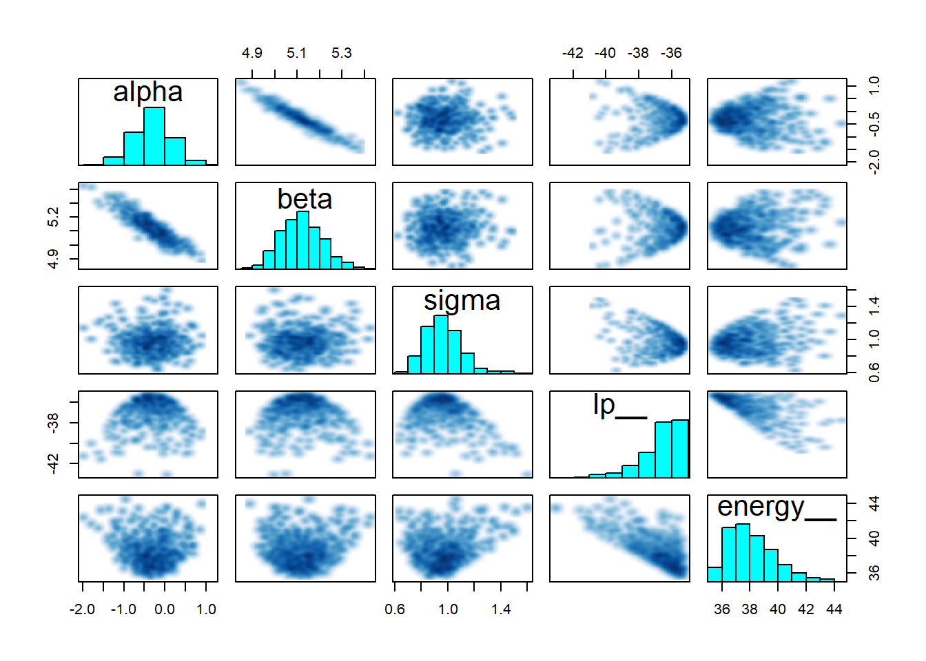

traceplot(robust_fit)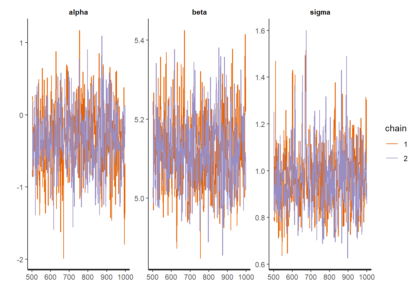

Everything looks pretty good! However, just for comparison, it might be interesting to compare these results to the maximum liklihood estimator approach:

mle_fit <- MASS::rlm(y ~ x, data = data)

summary(mle_fit)

## 
## Call: rlm(formula = y ~ x, data = data)
## Residuals:
##      Min       1Q   Median       3Q      Max 
## -2.01591 -0.69722  0.00958  0.65882 11.07708 
## 
## Coefficients:
##             Value Std. Error t value
## (Intercept) -0.42  0.52      -0.81  
## x            5.16  0.10      50.42  
## 
## Residual standard error: 1 on 48 degrees of freedom

So we achieved basically the same estimates for beta, which is good!