Multiple Linear Regression in Stan
Multiple Linear Regression
In this example I am going to practice multiple linear regression. Now I will add a second predictor to the model.
I’m going to go ahead and load rstan for use in this example
library(rstan)
rstan_options(auto_write = TRUE)
library(dplyr)
Generate Some Fake Data
Again, It is a good practice to generate some fake data to ensure that the model is behaving as expected.
x <- rnorm(40, 10, 5)
z <- rnorm(40, 0, 1)
pred <- data.frame(x = x, y = y)
noise <- rnorm(40,0,1)
y <- x*.5 + z * 0.25 + noise

data <- list( x= as.matrix(pred), y = y, N = length(x), K = 2L)
Specify the Model
The below Stan code models the familiar \(y = \beta_1*x + \beta_2*x + \alpha + \epsilon\)
Or more formally:
\[y_n \sim N(\alpha + \beta X_n,\sigma)\]
//multiple linear regression code
data {
  int<lower=0> N;   // number of data items
  int<lower=0> K;   // number of predictors
  matrix[N, K] x;   // predictor matrix
  vector[N] y;      // outcome vector
}
// this step does some transformations to the data
transformed data {
  matrix[N, K] Q_ast;
  matrix[K, K] R_ast;
  matrix[K, K] R_ast_inverse;
  // thin and scale the QR decomposition
  Q_ast = qr_Q(x)[, 1:K] * sqrt(N - 1);
  R_ast = qr_R(x)[1:K, ] / sqrt(N - 1);
  R_ast_inverse = inverse(R_ast);
}
parameters {
  real alpha;           // intercept
  vector[K] theta;      // coefficients on Q_ast
  real<lower=0> sigma;  // error scale
}
model {
  y ~ normal(Q_ast * theta + alpha, sigma);  // likelihood
}
// converts the quantities back to the original scale
generated quantities {
  vector[K] beta;
  beta = R_ast_inverse * theta; // coefficients on x
}
Modeling the Fake Data
So now we need to compile the Stan code. This takes a little while….
mult_linear_regression <- stan_model("stan_mult_linear_regression.stan")One that code has been compiled then we can actually fit the model. This is a simple model and it converges quickly (which it should).
fit1 <- sampling(mult_linear_regression, data = data, chains = 2, iter = 2000, refresh = 0)Now we can look at the model outputs with the summary which prints a lot of information or just look at the parameters one by one. I’m interested in if it could detect the true slope, in this case 0.5:
print(fit1, pars = "beta", probs = c(0.025, 0.5, 0.975))## Inference for Stan model: stan_mult_linear_regression.
## 2 chains, each with iter=2000; warmup=1000; thin=1;
## post-warmup draws per chain=1000, total post-warmup draws=2000.
##
## mean se_mean sd 2.5% 50% 98% n_eff Rhat
## beta[1] 0.46 0 0.03 0.39 0.46 0.53 1057 1
## beta[2] -0.13 0 0.07 -0.28 -0.13 0.00 798 1
##
## Samples were drawn using NUTS(diag_e) at Thu Jun 20 10:49:03 2019.
## For each parameter, n_eff is a crude measure of effective sample size,
## and Rhat is the potential scale reduction factor on split chains (at
## convergence, Rhat=1).Model Checking
As with any good Bayesian analysis it is important to perform some posterior checks to ensure that the model sufficiently converged. One check is the \(\hat{R}\) which is a measure of the mixing on the chaines with a target of one (which is achieved here).
Additionally, we can look at the trace plots to make sure everything converged and thise look good too.
traceplot(fit1)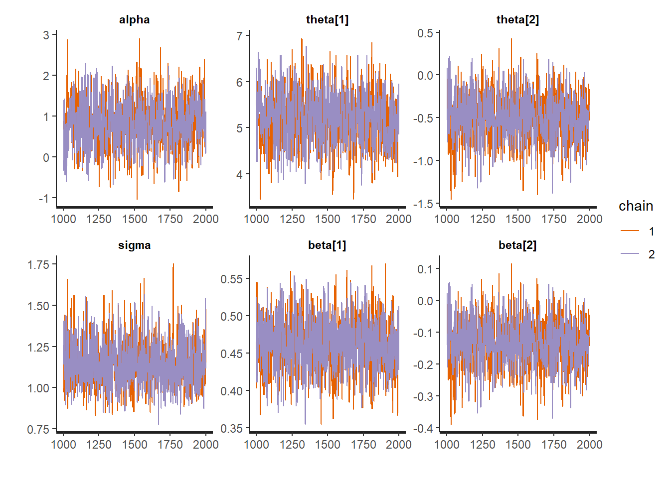
And finally a pairs plot which shows that sigma, alpha and beta all look reasonable centered with no strange patterns.
pairs(fit1)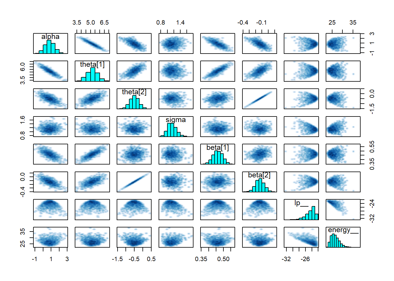
Fit on Actual Data
For the sake of illustration I am going to turn to our friend, mtcars to test this model. So first things first is to put our data into the correct format:
data <- list(y = mtcars$mpg, x = as.matrix(dplyr::select(mtcars, wt, disp)),
             N = nrow(mtcars), K = 2L)
Now we can fit the model with our already compiled Stan code and let it run.
fit_real <- sampling(mult_linear_regression, data = data, chains = 2, iter = 2000, refresh = 0)It fit the model without a problem. Now to view the outputs:
print(fit_real, pars = "beta", probs = c(0.025, 0.5, 0.975))## Inference for Stan model: stan_mult_linear_regression.
## 2 chains, each with iter=2000; warmup=1000; thin=1;
## post-warmup draws per chain=1000, total post-warmup draws=2000.
##
## mean se_mean sd 2.5% 50% 98% n_eff Rhat
## beta[1] -3.41 0.05 1.24 -5.73 -3.44 -0.99 597 1
## beta[2] -0.02 0.00 0.01 -0.04 -0.02 0.00 798 1
##
## Samples were drawn using NUTS(diag_e) at Fri Jun 21 13:09:10 2019.
## For each parameter, n_eff is a crude measure of effective sample size,
## and Rhat is the potential scale reduction factor on split chains (at
## convergence, Rhat=1).The \(\hat{R}\) are at one so it doesn’t look too bad. Of course a better practice would be to run this model a little longer and supply strong priors because the effect number of samples is somewhat small. But another model nonetheless.
We can also visualise the outputs using the bayesplot package
posterior <- as.array(fit_real)

bayesplot::mcmc_intervals(posterior, pars = c("beta[1]","beta[2]", "sigma"))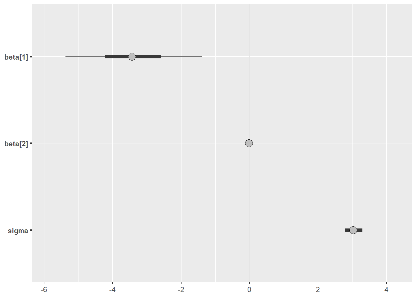
Research and Methods Resources
me.dewitt.jr@gmail.com
Winston- Salem, NC
Copyright © 2018 Michael DeWitt. All rights reserved.