Autoregressive Modeling in Stan

This post looks at modeling autoregressive models. Autoregression is typically important when dealing with time series analysis. The general idea is that the past value of a repeatedly measured item will be indicative of its future value. A good example is a stock. Today’s stock price could be modelled as a function of yesterday’s stock price. While this isn’t entirely true, it does approximate a decent model.

Data Generating Process

In this case I am going to look at an AR(3) model. Thus the model form would take on the following data generating process:

\[y_n \sim N(\alpha + \beta_1y_{n-1} + \beta_2y_{n-2} + \beta_3y_{n-3}, \sigma)\]

And we can used a built in feature of R to help us simulate these data. Note that I have not specificed a moving average.

fake_data <-arima.sim(n = 200, model = list(ar = c(.2, .5, .05)))

ts.plot(fake_data, main = "Time Series Plot of Our Fake Data")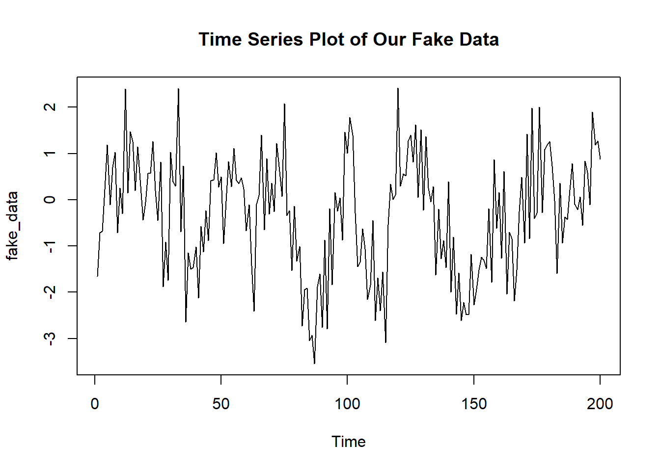

Stan

The Model

writeLines(readLines("stan_ar_models.stan"))

// From https://mc-stan.org/docs/2_18/stan-users-guide/autoregressive-section.html
// Allowing for flexible autoregression for time series modeling

data {
  int<lower=0> K;  // Order of Autoregression
  int<lower=0> N; // number of observations
  real y[N];      // Outcome
}
parameters {
  real alpha;
  real beta[K];
  real sigma;
}
model {
  for (n in (K+1):N) {
    real mu = alpha;
    for (k in 1:K)
      mu += beta[k] * y[n-k];
    y[n] ~ normal(mu, sigma);
  }
}

The Modeling Process

library(rstan)

rstan_options(auto_write = TRUE)
model <- stan_model("stan_ar_models.stan")

Format Data

Now we need to format our data for our Stan program:

stan_dat <- list(
  N = length(fake_data),
  K = 3,
  y = as.vector(fake_data)
)

Fit the Model

Let’s run our model with the usual conditions.

fit <- sampling(model, stan_dat,
                cores = 2, iter = 1000,
                refresh = 0, chains = 2)

Model Checking

And as always special thanks to Michael Betancourt for these amazing tools for diagnostics.

util <- new.env()
source('stan_utilities.R', local=util)

util$check_all_diagnostics(fit)

Inference

print(fit, pars = "beta")

## Inference for Stan model: stan_ar_models.
## 2 chains, each with iter=1000; warmup=500; thin=1; 
## post-warmup draws per chain=500, total post-warmup draws=1000.
## 
##         mean se_mean   sd  2.5%   25%  50%  75%  98% n_eff Rhat
## beta[1] 0.23       0 0.07  0.09  0.18 0.23 0.28 0.37  1126    1
## beta[2] 0.52       0 0.07  0.40  0.47 0.52 0.56 0.65  1137    1
## beta[3] 0.00       0 0.07 -0.13 -0.05 0.00 0.05 0.15   831    1
## 
## Samples were drawn using NUTS(diag_e) at Thu Jun 20 10:10:34 2019.
## For each parameter, n_eff is a crude measure of effective sample size,
## and Rhat is the potential scale reduction factor on split chains (at 
## convergence, Rhat=1).

Research and Methods Resources
me.dewitt.jr@gmail.com

Winston- Salem, NC

Michael DeWitt