A Normal- Normal Hierarchical Model

Our Data

The example in the book utilises data from the US Department of Commerce’s Survey of Current Business. The data contain information by quarter from 1979 to 1989. After some hunting I found that Dr Gill graciously put the data to this book in the BaM package which I subsequently downloaded from CRAN.

data_sales <- BaM::retail.sales

And we can inspect it a little more:

data_sales

To describe the data further:

• DSB - National Wage and Incime Disbursements (Billions)
• EMP - Employees on non-agricultural payrolls (thousands)
• BDG - building dealer sales (millions)
• CAR - car dealer sales (millions)
• FRN - home furnishings dealer sales (millions)
• GRM - general merchanise sales in millions

Generative Model

In the case of the model for the data it is specified as

\[y_{i,j} \sim N(\beta_0[i]+\beta_1[i]x_j, \tau)\] \[\beta_0[i] \sim N(\mu_{\beta.0},\tau_{\beta.0})\] \[\beta_1[i] \sim N(\mu_{\beta.1},\tau_{\beta.1})\] \[\tau\sim\Gamma(0.01, 0.01)\]

Now to Stan

To implement the above model we would need to do the following:

// Normal Normal Model

data {
  int<lower=0> J;   // number of data items
  int<lower=0> I;   // number of predictors
  vector[J] x; // depdent variable
  matrix[J, I] y;   // predictor matrix
}
parameters {
  vector[I] beta0; //vector of beta0s
  vector[I] beta1; //vector of beta1s
  real mu_beta0; //average value of beta0
  real mu_beta1; //average value of beta1
  real tau;
  real tau_beta1;
  real tau_beta0;
  
}

transformed parameters{
  real xbar;
  xbar = mean(x); // calculate the average value of x
  
}
model {
  // priors
  tau ~ gamma(.01, .01); 
  mu_beta0 ~ normal(0, 10);
  tau_beta0 ~ gamma( .01, .01);
  mu_beta1 ~ normal(0, 10);
  tau_beta1 ~ gamma( .01, .01);
  
  //group effects for each indicator
  for(i in 1:I){
  beta0[i] ~ normal(mu_beta0, tau_beta0);
  beta1[i] ~ normal(mu_beta1, tau_beta1);
  }
  
  //model
  for(j in 1:J){
    y[j]~ normal(beta0 + beta1*(x[j]-xbar), tau);
  }
  
}

Now we can make sure that the model compiles.

library(rstan)
rstan_options(auto_write = TRUE)
nn_fit <- stan_model("stan_hlm_nn.stan")

Format our data for the modelL

data <- list(J = nrow(data_sales),
             I = 6L,
             x = data_sales$TIME,
             y = as.matrix(data_sales[,-1])/1000)

And fit our model:

fit <- sampling(nn_fit, data = data,  chains = 2, iter = 2000, refresh = 0)

Looking at the output from our model it matches that on page 405 in the second edition almost right on! Hooray!

print(fit, probs = c(0.025, 0.5, 0.975))

## Inference for Stan model: stan_hlm_nn.
## 2 chains, each with iter=2000; warmup=1000; thin=1; 
## post-warmup draws per chain=1000, total post-warmup draws=2000.
## 
##              mean se_mean    sd    2.5%     50%     98% n_eff Rhat
## beta0[1]     1.86    0.02  0.75    0.34    1.85    3.32  2144    1
## beta0[2]    96.33    0.02  0.75   94.81   96.34   97.84  2387    1
## beta0[3]    17.09    0.02  0.79   15.59   17.08   18.63  2342    1
## beta0[4]    66.06    0.02  0.75   64.57   66.04   67.57  2446    1
## beta0[5]    16.18    0.01  0.75   14.75   16.16   17.72  2662    1
## beta0[6]    37.88    0.01  0.75   36.40   37.88   39.36  2652    1
## beta1[1]     0.04    0.00  0.06   -0.08    0.04    0.16  2127    1
## beta1[2]     0.50    0.00  0.06    0.37    0.50    0.62  2754    1
## beta1[3]     0.32    0.00  0.05    0.21    0.32    0.42  2315    1
## beta1[4]     1.52    0.00  0.06    1.40    1.52    1.64  2489    1
## beta1[5]     0.37    0.00  0.06    0.25    0.37    0.48  2407    1
## beta1[6]     0.55    0.00  0.06    0.43    0.55    0.68  2540    1
## mu_beta0     9.66    0.21  9.92   -9.79    9.78   28.89  2259    1
## mu_beta1     0.55    0.01  0.27    0.04    0.55    1.10  1890    1
## tau          4.97    0.00  0.22    4.56    4.96    5.44  2401    1
## tau_beta1    0.62    0.02  0.30    0.31    0.55    1.35   359    1
## tau_beta0   48.00    0.51 16.72   25.95   44.68   89.76  1086    1
## xbar        22.50     NaN  0.00   22.50   22.50   22.50   NaN  NaN
## lp__      -587.03    0.13  3.35 -594.79 -586.69 -581.76   697    1
## 
## Samples were drawn using NUTS(diag_e) at Fri Jun 21 13:08:23 2019.
## For each parameter, n_eff is a crude measure of effective sample size,
## and Rhat is the potential scale reduction factor on split chains (at 
## convergence, Rhat=1).

Posterior Model Checking

Thus we refit this model in Stan, but let’s check the trace plots and some posterior predictive checks to make sure we have a model that makes sense.

traceplot(fit, "beta0")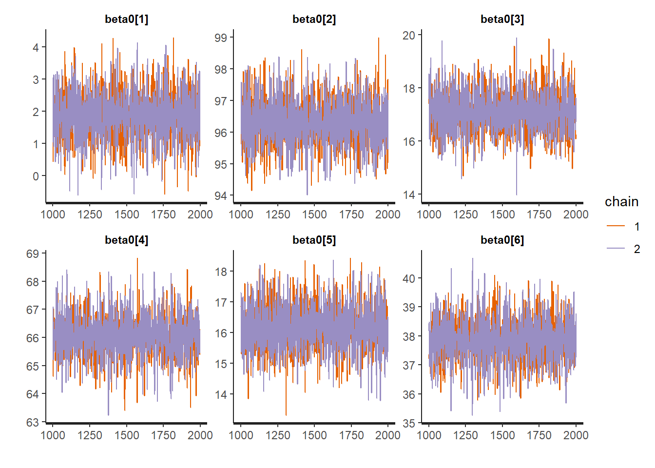

traceplot(fit, "beta1")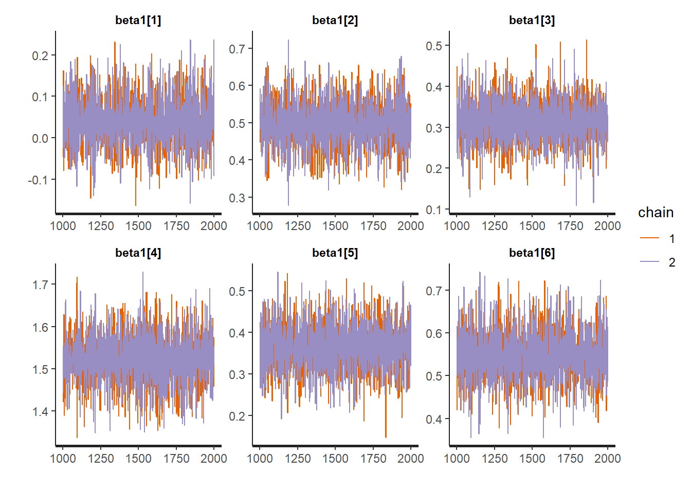

library(bayesplot)
posterior <- as.array(fit)

mcmc_areas(posterior,
           pars = c("beta1[1]","beta1[2]","beta1[3]","beta1[4]","beta1[5]","beta1[6]"),
           prob = 0.8)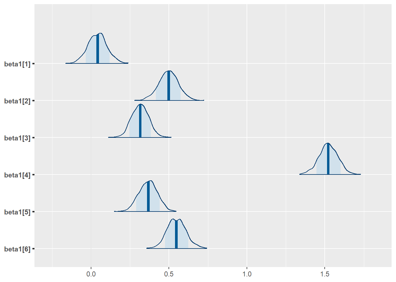

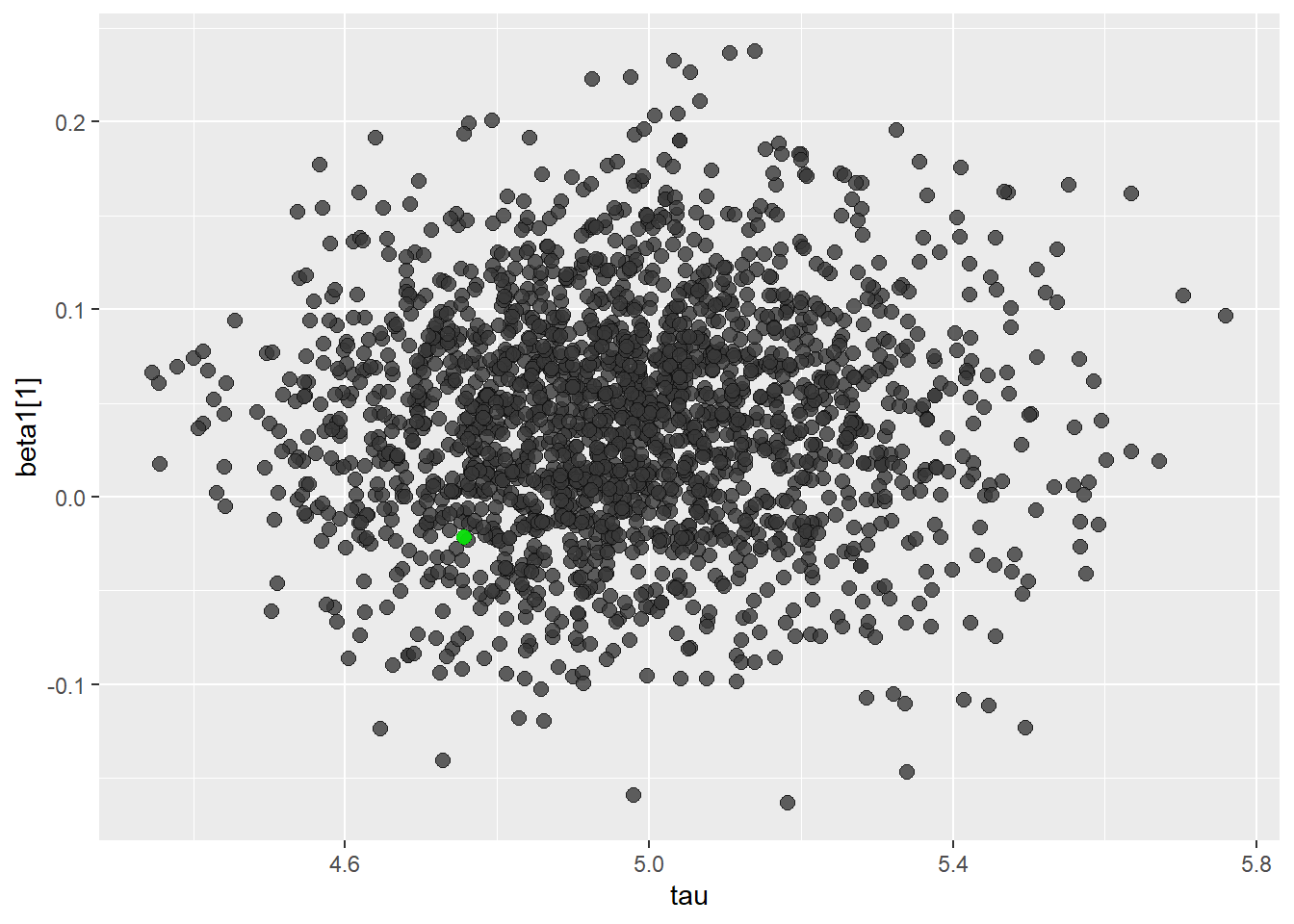
posterior2 <- extract(fit, inc_warmup = TRUE, permuted = FALSE)

color_scheme_set("darkgray")
mcmc_scatter(
  as.matrix(fit),
  pars = c("tau", "beta1[1]"), 
  np = nuts_params(fit), 
  np_style = scatter_style_np(div_color = "green", div_alpha = 0.8)
)