Linear Regression in Stan

My Mission

Write a bunch of Stan Code to practice building models in Stan. While brms is fantastic, I feel like I need to put in the work to learn to build the Stan code myself. I am going to try and work through one of the exercises each day from the handbook and other websites dealing with interesting models.

Linear Regression

Linear regression is pretty much the cornerstone of models, so it is a good place to start.

I’m going to go ahead and load rstan for use in this example

library(rstan)
rstan_options(auto_write = TRUE)

Generate Some Fake Data

One of the most important processes in any model fitting data is to generate some data before hand. If your model performs as expected on the fake data simulation then you can have confidence that your model will work when faced with your actual data.

I’m going to generate data from a normal distribution and a noise parameter. My slope will be set at 0.5.

x <- rnorm(40, 10, 5)
noise <- rnorm(40,0,1)
y <- x*.5 + noise

data <- list( x= x, y = y, N = length(x))

Specify the Model

The below Stan code models the familiar \(y = \beta*x + \alpha + \epsilon\)

Or more formally:

\[y_n \sim N(\alpha + \beta X_n,\sigma)\]

data {
  int<lower=0> N;
  vector[N] x;
  vector[N] y;
}
parameters {
  real alpha;
  real beta;
  real<lower=0> sigma;
}
model {
  y ~ normal(alpha + beta * x, sigma);
}

Modeling the Fake Data

So now we need to compile the Stan code. This takes a little while….

linear_regression <- stan_model("stan_linear_regression.stan")

One that code has been compiled then we can actually fit the model. This is a simple model and it converges quickly (which it should).

fit1 <- sampling(linear_regression, data = data, chains = 2, iter = 1000, refresh = 0)

Now we can look at the model outputs with the summary which prints a lot of information or just look at the parameters one by one. I’m interested in if it could detect the true slope, in this case 0.5:

print(fit1, pars = "beta", probs = c(0.025, 0.5, 0.975))

## Inference for Stan model: stan_linear_regression.
## 2 chains, each with iter=1000; warmup=500; thin=1; 
## post-warmup draws per chain=500, total post-warmup draws=1000.
## 
##      mean se_mean   sd 2.5%  50%  98% n_eff Rhat
## beta 0.51       0 0.03 0.44 0.51 0.58   324    1
## 
## Samples were drawn using NUTS(diag_e) at Thu Jun 20 10:47:33 2019.
## For each parameter, n_eff is a crude measure of effective sample size,
## and Rhat is the potential scale reduction factor on split chains (at 
## convergence, Rhat=1).

And it did a reasonable job! Yahoo it worked.

Model Checking

As with any good Bayesian analysis it is important to perform some posterior checks to ensure that the model sufficiently converged. One check is the \(\hat{R}\) which is a measure of the mixing on the chaines with a target of one (which is achieved here).

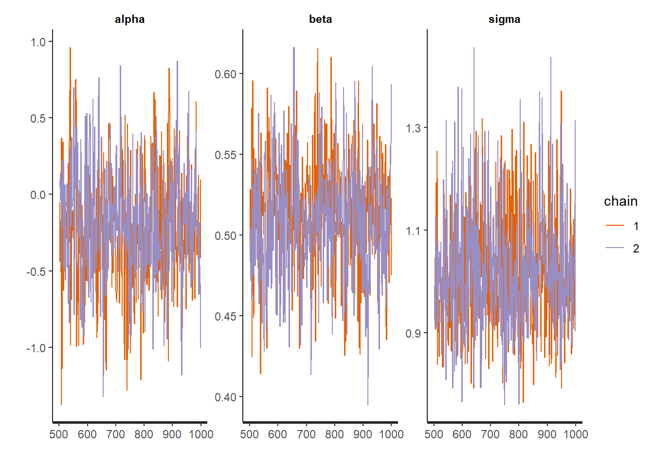
Additionally, we can look at the trace plots to make sure everything converged and thise look good too.

traceplot(fit1)

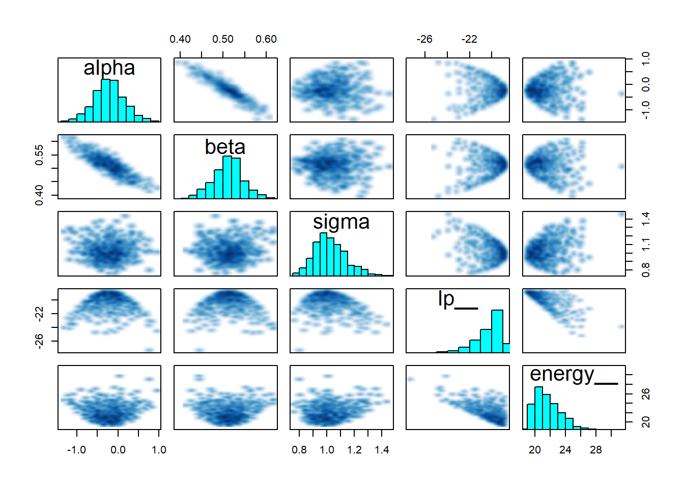
And finally a pairs plot which shows that sigma, alpha and beta all look reasonable centered with no strange patterns.

pairs(fit1)

So, yahoo! first real model in Stan!