library(deSolve)
library(tidyverse)5 Dynamics of Immune Response
Nowak and May (Nowak and May 2000) argue that:
- virus load is an important determinant of disease
- immune responses limit virus load
- individual variation in immune responsiveness accounts for much of the observed variation in the outcome of a disease
5.1 Predator-Prey Dynamics of the Immune System
We extend the basic model with a cytotoxic T lymphocyte (CTL) response \(z\), which kills infected cells at rate \(p\). In the simplest case the CTL are produced at a constant rate \(c\) and decay at rate \(b\), independent of antigen.
\[ \frac{dx}{dt} = \lambda - dx - \beta x v \] \[ \frac{dy}{dt} = \beta x v - ay - pyz \\ \] \[ \frac{dv}{dt} = ky - uv \] \[ \frac{dz}{dt} = c -bz \\ \]
With the basic reproduction number defined for this system as
\[ R_0 = \frac{\beta \lambda k}{adu} \]
And the basic reproduction number in the presence of an immune response (CTL)
\[ R_1 = \frac{\beta \lambda k}{(a +a')du} \]
Where:
\[ a' = \frac{cp}{b} \]
representing the rate at which infected cells are eliminated by the CTL response at equilibrium.
If \(R_1 < 1\) then the infection will clear. The virus may spread initially, but once the immune response is activated, each infected cell will on average give rise to less than one newly infected cell and thus the infection will die out.
5.2 Simulating the Immune Response
We code the four-compartment system and reuse the contact and replication parameters from the basic model, adding the CTL killing rate \(p\), production rate \(c\), and decay rate \(b\).
immune_ode <- function(time, state, parameters){
with(as.list(c(state, parameters)),{
dx <- lambda - d * x - beta * x * v
dy <- beta * x * v - a * y - p * y * z
dv <- k * y - u * v
dz <- c - b * z
return(list(c(dx, dy, dv, dz)))
})
}
t <- seq(0, 30, .1)
params <- c(
lambda = 1e5, # Uninfected cell production rate
d = .1, # Cell death rate
a = .5, # Infected cell death rate
beta = 2e-7, # Rate constant
k = 100, # Virus production from infected cell
u = 5, # Free virus lifespan
p = 1, # CTL killing rate
c = .1, # CTL production rate
b = .05 # CTL decay rate
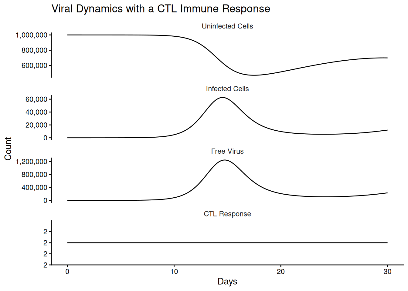
)The constant-production assumption gives an equilibrium CTL level of \(\hat{z} = c/b\), so we can compute the two reproductive ratios directly and confirm that the immune response lowers, but does not here eliminate, viral spread.
a_prime <- with(as.list(params), c * p / b)

R0 <- with(as.list(params), beta * lambda * k / (a * d * u))
R1 <- with(as.list(params), beta * lambda * k / ((a + a_prime) * d * u))

c(R0 = R0, R1 = R1)
R0 R1
8.0 1.6 x0 <- unname(params["lambda"] / params["d"])
init <- c(x = x0, y = 1, v = 1, z = unname(params["c"] / params["b"]))
out <- ode(init, t, immune_ode, params)
out_df <- as_tibble(as.data.frame(out))compartment_names <- c("Uninfected Cells",
"Infected Cells",
"Free Virus",
"CTL Response")
p_plot <- out_df %>%
setNames(c("time", compartment_names)) %>%
gather(compartment, value, -time) %>%
mutate(compartment = factor(compartment, compartment_names)) %>%
ggplot(aes(time, y = value)) +
geom_line() +
facet_wrap(~compartment, ncol = 1, scales = "free_y") +
theme_classic() +
labs(
title = "Viral Dynamics with a CTL Immune Response",
x = "Days",
y = "Count"
) +
scale_y_continuous(labels = scales::comma_format(accuracy = 1)) +
theme(strip.background = element_blank())
p_plot