2 The Basic Model of Virus Dynamics

library(deSolve)
library(tidyverse)

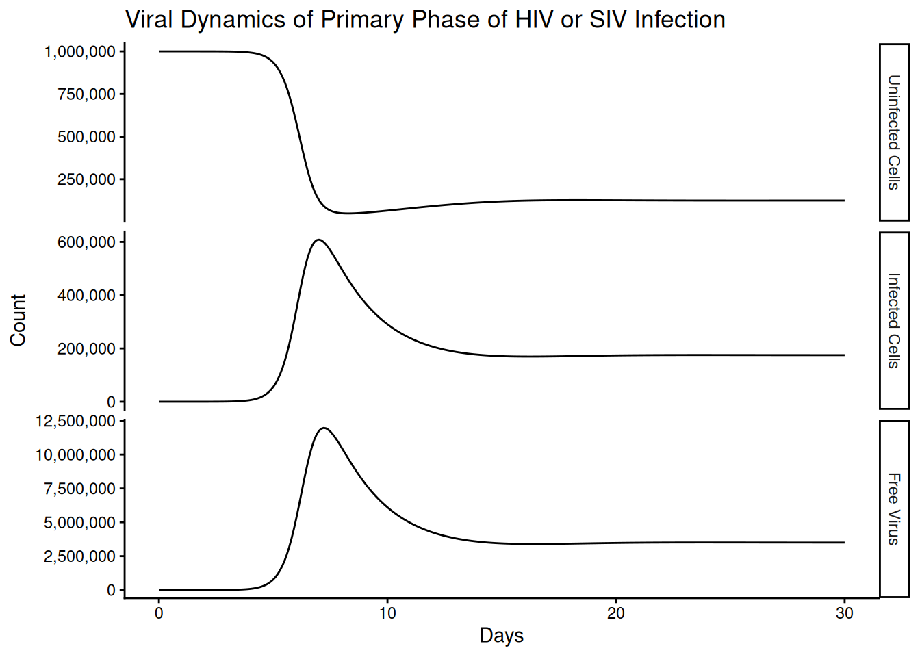
The basic model of virus dynamics (Nowak and May 2000) tracks three populations: uninfected target cells \(x\), infected cells \(y\), and free virus particles \(v\). Uninfected cells are produced at a constant rate \(\lambda\), die at rate \(d\), and become infected on contact with virus at rate \(\beta\). Infected cells die at rate \(a\), and each produces free virus at rate \(k\), which is in turn cleared at rate \(u\).

\[ \frac{dx}{dt} = \lambda - dx - \beta x v \] \[ \frac{dy}{dt} = \beta x v - a y \] \[ \frac{dv}{dt} = k y - u v \]

The basic reproductive ratio of the virus, the average number of newly infected cells arising from one infected cell placed in a fully susceptible cell population, is

\[ R_0 = \frac{\beta \lambda k}{a d u} \]

The virus can establish an infection only if \(R_0 > 1\).

2.1 Set Up the ODE

base_ode <- function(time, state, parameters){
    with(as.list(c(state, parameters)),{
        
        dx <- lambda - d*x - beta * x * v
        dy <- beta * x * v - a * y
        dv <- k * y - u * v
        
        return(list(c(dx,dy,dv)))
    })
    
}

t <- seq(0,30,.1)

params <- c(
    lambda =1e5,# Uninfected cell production rate
    d = .1, # Cell Death Rate
    a = .5, # Infected Cell Death Rate
    beta = 2e-7, # "Rate Constant"
    k = 100, # Virus production from infected cell
    u = 5 # Free virus lifespan
)

2.2 Solve the System

Guessing initial values from a graph:

x0 <- params["lambda"][1]/params["d"][1]
init <- c(x = unname(x0), 
                    y = 1, v = 1)

out <- ode(init, t, base_ode, params)

out_df <- as_tibble(as.data.frame(out))

Note that the differences in the scales across compartments are reproduced almost immediately, as in the book.

compartment_names <- c("Uninfected Cells",
"Infected Cells",
"Free Virus")

p <- out_df %>% 
    setNames(c("time", compartment_names)) %>% 
    gather(compartment, value, -time) %>% 
    mutate(compartment = factor(compartment, compartment_names)) %>% 
    ggplot(aes(time, y = value))+
    geom_line()+
    facet_grid(rows = vars(compartment),scales = "free_y")+
    theme_classic()+
    labs(
        title = "Viral Dynamics of Primary Phase of HIV or SIV Infection",
        x = "Days",
        y = "Count"
    )+
    scale_y_continuous(labels = scales::comma_format(accuracy = 1000))

p