library(deSolve)
library(tidyverse)3 Anti-viral Drug Therapy
From pages 35-37.
3.1 Set Up the ODE
Represents infected cells becoming:
- Latently infected: do not produce new virions, but contain replication competent virus that can be re-activated to become virus producing
- long-lived chronic producers: produce small amounts of virus over long periods
- cells which harbor defective provirus
These dynamics can be represented by the below equations:
\[ \frac{dx}{dt} = \lambda - dx - \beta x v \\ \] \[ \frac{dy_1}{dt} = q_1 \beta x v-a_1y_1+\alpha y_2 \\ \] \[ \frac{dy_2}{dt} = q_2 \beta x v-a_2y_2-\alpha y_2 \\ \] \[ \frac{dy_3}{dt} = q_3 \beta x v-a_3y_3 \\ \] \[ \frac{dv}{dt} = k y_1 - u v \]
These equations can then be coded as follows:
base_ode <- function(time, state, parameters){
  with(as.list(c(state, parameters)),{

    dx <- lambda - d*x - beta * x * v
    dy1 <- q1*beta * x * v - a1 * y1 + alpha * y2
    dy2 <- q2*beta * x * v - a2 * y2 - alpha * y2
    dy3 <- q3*beta * x * v - a3 * y3
    dv <- k * y1 - u * v

    return(list(c(dx, dy1, dy2, dy3, dv)))
  })

}
Now we can set up the initial conditions and constants to simulate the outputs from this system of equations.
t <- seq(0,30,.1)

params <- c(
  lambda =1e7,# Uninfected cell production rate
  d = .1, # Cell Death Rate
  a1 = .5, # Infected Cell Death Rate
  a2 = .01, # Infected Cell Death Rate
  a3 = .008, # Infected Cell Death Rate
  beta = 5e-10, # "Rate Constant"
  alpha = .3, # Virus Production rate of reactivated latent
  k = 500, # Virus production from infected cell
  u = 5, # Free virus lifespan
  q1 = .55, # P(Infected State | Infected)
  q2 = .05, # P(Latent State | Infected)
  q3 = .4 # P(Defective Provirus | Infected)
)

#' Guessing Initial values from a graph
x0 <- params["lambda"][1]/params["d"][1]
init <- c(x = unname(x0),
          y1 = 1,y2=0,y3=0, v = 1)

out <- ode(init, t, base_ode, params)

out_df <- as_tibble(as.data.frame(out))
As before, the differences in the scales across compartments are reproduced almost immediately, as in the book.
compartment_names <- c("Uninfected Cells",
"Actively Infected Cells",
"Latently Infected Cells",
"Cells Infected with Defective Virus",
"Free Virus")

p <- out_df %>%
  setNames(c("time", compartment_names)) %>%
  gather(compartment, value, -time) %>%
  mutate(compartment = factor(compartment,
                              compartment_names)) %>%
  ggplot(aes(time, y = value))+
  geom_line()+
  facet_wrap(~compartment, ncol = 1,scales = "free_y")+
  theme_classic()+
  labs(
    title = "Viral Dynamics of Primary Phase of HIV or SIV Infection",
    x = "Days",
    y = "Count"
  )+
  scale_y_continuous(labels = scales::comma_format(accuracy = 1000))+
  theme(strip.background = element_blank())

p 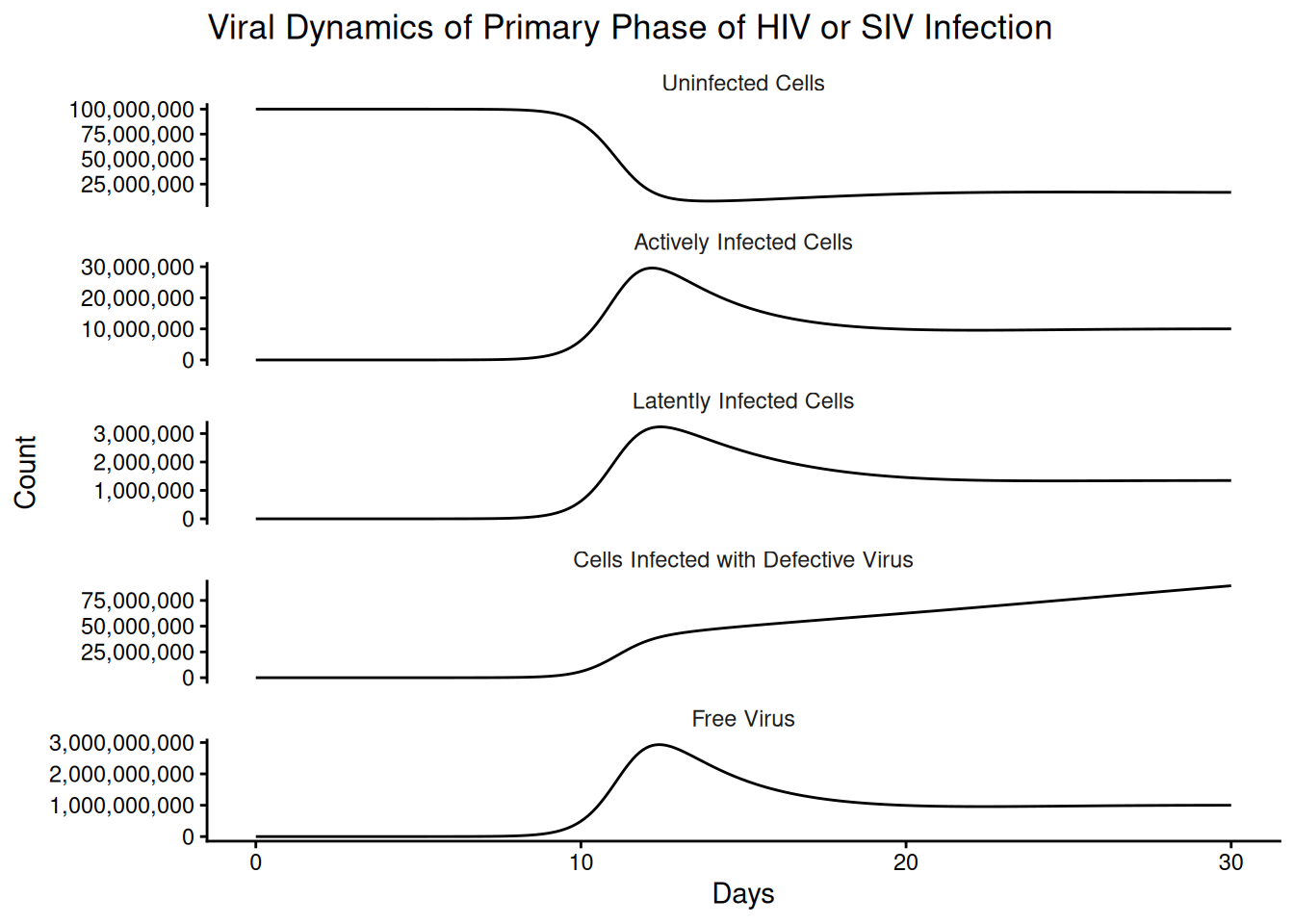
3.1.1 Equilibrium Conditions
\[ \hat{x} = \frac{x_0}{R_0} \\ \] \[ \hat{y_1} = (R_0-1)\frac{du}{\beta k} = \hat{v}\frac{u}{k} \\ \] \[ \hat{y_2}=\frac{\hat{y_1}\frac{a_1}{q_1}}{\frac{\alpha +a_2}{q_2}+\frac{\alpha}{q_1}}\\ \] \[ \hat{y_3} = \hat{y_2} \frac{\frac{\alpha + a_2}{q_2}}{\frac{a_3}{q_3}}\\ \] \[ \hat{v} = (R_0-1)\frac{d}{\beta} \]
With \(R_0\) given by:
\[ R_0 = \frac{\beta \lambda \ k}{a_1du}(q_1+q_2 \frac{\alpha}{\alpha + a_2}) \]
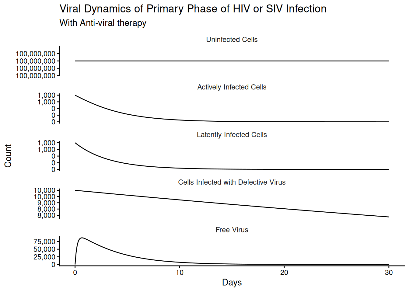
3.2 Effect of Anti-Virals
The big take-away from these equations is that introduction of an anti-viral should reduce the contact rate, \(\beta\), to zero (or some much lower value).
params["beta"] <- 0

init <- c(x = unname(x0),
          y1 = 1000,y2=1000,y3=10000, v = 50)

out_antiviral <- ode(init, t, base_ode, params)

out_df_av <- as_tibble(as.data.frame(out_antiviral))
p <- out_df_av %>%
setNames(c("time", compartment_names)) %>%
gather(compartment, value, -time) %>%
mutate(compartment = factor(compartment,
compartment_names)) %>%
ggplot(aes(time, y = value))+
geom_line()+
facet_wrap(~compartment, ncol = 1,scales = "free_y")+
theme_classic()+
labs(
title = "Viral Dynamics of Primary Phase of HIV or SIV Infection",
subtitle = "With Anti-viral therapy",
x = "Days",
y = "Count"
)+
scale_y_continuous(labels = scales::comma_format(accuracy = 1000))+
theme(strip.background = element_blank())
p