Nowcasting

1 Introduction

Now I want to write quickly about nowcasting. What is nowcasting? It is the process of modeling data that we get on a faster frequency in order to anticipate the true underlying data that we may get on a longer frequency. A perfect example of this is the GDP. Here we get GDP information quarterly, but we get data regarding other economic activity monthly (or faster). So let’s try!

2 Data

First, I am going to pull data using the fredr package to pull data regarding the GDP, Employment, and Industrial production. In each case I will pull the each metric in percent change from the previous measure.

# Billions of Dollars
gdp_dat <- fredr(series_id = "GDPC1",
                                 observation_start = as.Date("1950-01-01"), units = "pch")

# All Employees
allemp <- fredr(series_id = "PAYEMS", 
                                observation_start = as.Date("1950-01-01"), units = "pch")

# Industrial Production
industrial_prod <- fredr(series_id = "INDPRO", 
                                observation_start = as.Date("1950-01-01"), units = "pch")

3 Model

Now we can build out model. Nowcasting using a state-space model that takes the form of predicting GDP, first by estimating a latent state for GDP denoted by \(x\), using the previous state’s value and a matrix of new predictors (\(Z\)). This will then be used to predict the actual value of GDP, \(y\).

\[x_i \sim N(\alpha + X_{i-1}+\bf{Z}\gamma, \sigma_{\eta})\] \[y_i\sim N(x_i, \sigma_{\epsilon})\]

We also specify fairly vague priors that could be refined (or we could specify hyperpriors which are learned from the data).

3.1 In Stan

Now we can code this up in Stan. Here I am taking inspiration from @nowcastingStan with a few tweaks.

writeLines(readLines("nowcast.stan"))

data {
  int N1; // length of low frequency series
  int N2; // length of high frequency series
  int K;
  int freq; // every freq-th observation of the high frequency series we get an observation of the low frequency one
  vector[N1] y;
  matrix[N2, K] z;
}
parameters {
  real<lower = 0> sigma_epsilon;
  real<lower = 0> sigma_eta;
  vector[K] gamma;
  real alpha;
  vector[N2] x;
}
model {
  int count;
  // priors
  sigma_epsilon ~ cauchy(0,1);
  sigma_eta ~ cauchy(0,1);
  gamma ~ normal(0,1);

  // likelihood
  count = 0;
  for(i in 2:N2){
    target += normal_lpdf(x[i]| alpha + x[i-1] + z[i,]*gamma, sigma_eta);
    if(i%freq==0){
      count = count + 1;
      target += normal_lpdf(y[count]| x[i], sigma_epsilon);
    }
  }
}

Now we can compile the model.

library(rstan)
options(mc.cores = parallel::detectCores())
rstan_options(auto_write = TRUE)

model_nowcast <- stan_model("nowcast.stan")

We also need to format our data for Stan.

model_data <- list(N1 = length(gdp_dat$value), 
                   N2 = nrow(allemp), 
                   freq = 4L, 
                   y = gdp_dat$value, 
                                     K = 2,
                   z = as.matrix(cbind(allemp$value, industrial_prod$value)))

Now we can run the model. Note that this will take a little while to run because of the number of iterations required. I’ve set the max_treedepth argument to 15 which allows the algorithm to explore the posterior space before turning.

fit <- sampling(model_nowcast, 
                                data = model_data, 
                                chains = 2, iter = 10000, refresh = 0,
                                control = list(max_treedepth = 15),
                                seed = 42)

4 Results

Now we can examine our outputs:

print(fit, pars = c("alpha", "gamma"))

## Inference for Stan model: nowcast.
## 2 chains, each with iter=10000; warmup=5000; thin=1; 
## post-warmup draws per chain=5000, total post-warmup draws=10000.
## 
##           mean se_mean   sd  2.5%   25%   50%   75% 97.5% n_eff Rhat
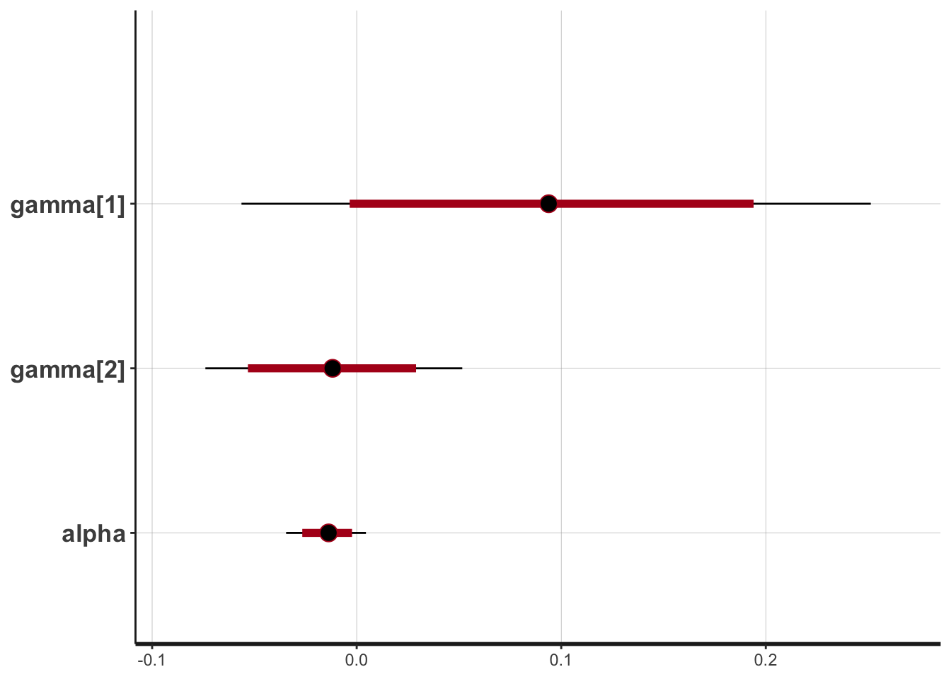
## alpha    -0.01       0 0.01 -0.03 -0.02 -0.01 -0.01  0.00  7129    1
## gamma[1]  0.09       0 0.08 -0.06  0.04  0.09  0.14  0.25  6959    1
## gamma[2] -0.01       0 0.03 -0.07 -0.03 -0.01  0.01  0.05 11945    1
## 
## Samples were drawn using NUTS(diag_e) at Tue Jan 21 16:48:36 2020.
## For each parameter, n_eff is a crude measure of effective sample size,
## and Rhat is the potential scale reduction factor on split chains (at 
## convergence, Rhat=1).

And visualize said outouts. Note that zero is included in the posterior intervals for these predictors indicating that these might not be the best for predicting GDP.

stan_plot(fit, pars = c("gamma", "alpha"))

out <- as.data.frame(fit, pars = "x")

out_long <- out %>% 
    gather(iter, time) %>% 
    group_by(iter) %>% 
    summarise(lower = quantile(time, probs = .025),
                        median = quantile(time, probs = .5),
                        upper = quantile(time, probs = .975)) %>% 
    mutate(index = parse_integer(str_extract(iter, "\\d{1,4}"))) %>% 
    arrange(index) %>% 
    add_column(date = allemp$date)

out_long %>% 
    ggplot(aes(date))+
    geom_ribbon(aes(ymin = lower, ymax = upper), alpha = .5, fill = uncg_pal[[2]])+
    scale_x_date()+
    geom_point(data = gdp_dat, aes(date, value), color = uncg_pal[[1]])+
    labs(
        title = "Nowcasting US GDP",
        subtitle = "Using Employment\nIndustrial Product Monthly Perc Change",
        y = "GDP",
        x = NULL
    )

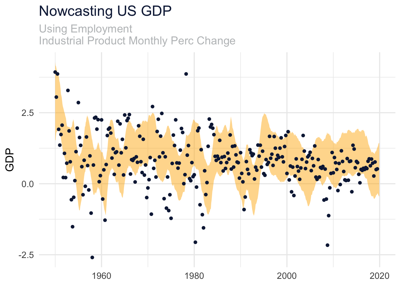
It looks our model does fairly well in predicting GDP, at least since 2015 or so!

---

Intermediate Macroeconomics
me.dewitt.jr@gmail.com

Code licensed under the BSD 3-clause license
Text licensed under the CC-BY-ND-NC 4.0 license

See the Repository

Copyright © 2020 Michael DeWitt