Labor Productivity

1 Introduction

In this post we examine the historical labor productivity for the United States.

2 Data

First we will pull Gross Domestic Product (GDP) using the Federal Reserve fredr API. Additionally, we can pull the civilian employment level. Note that these two measures are on different scales and recorded in different units (billions of USD for GDP and thousands of persons for employment).

# Billions of Dollars
gdp_dat <- fredr(series_id = "GDPC1",
                                 observation_start = as.Date("1950-01-01"))

# Civilian Employment Level
# Thousands of Persons
allemp <- fredr(series_id = "LNU02000000", 
                                observation_start = as.Date("1950-01-01"))

Now we want the last quarter for GDP and the last month for employment. This will be used to calculate a yearly productivity value.

gdp_q4 <- gdp_dat %>% 
    group_by(year = lubridate::year(date)) %>% 
    filter(date == min(date)) %>% 
    ungroup() %>% 
    rename(gpd = value)

emp_q4 <- allemp %>% 
    group_by(year = lubridate::year(date)) %>% 
    filter(date == min(date)) %>% 
    ungroup() %>% 
    rename(labor = value)

combined_dat <- gdp_q4 %>% 
    select(date, year, gpd) %>% 
    left_join(emp_q4 %>% 
                            select(date, year, labor))

3 Analysis

To answer the question about productivity growth, we need to perform the following operations:

1. Calculate the labor productivity by dividing GDP by employment (which basically indicates how much value is created per capita)
   
2. Calculate the percent change year over year in productivity

3.1 Calculate Percent Change

dat_productivity <- combined_dat %>% 
    ungroup() %>% 
    mutate(productivity = gpd/labor) %>% 
    mutate(delta_productivity = (productivity - lag(productivity, 1, default = 0))/lag(productivity, 1, default = ))

3.2 Plotting by Year

Now we can plot the productivity percent change year over year as shown below.

dat_productivity %>% 
    ggplot(aes(date, delta_productivity))+
    geom_line(color = uncg_pal[[1]])+
    geom_hline(yintercept = 0, lty = "dashed", color = "red")+
    scale_x_date(breaks = "4 year", date_labels =  "%y")+
    labs(
        title = "Year over Year Average Labor Productivity",
        subtitle = "Since 1950",
        caption = "Data: FRED St. Louis Federal Reserve"
    )+
    scale_y_continuous(labels = scales::percent)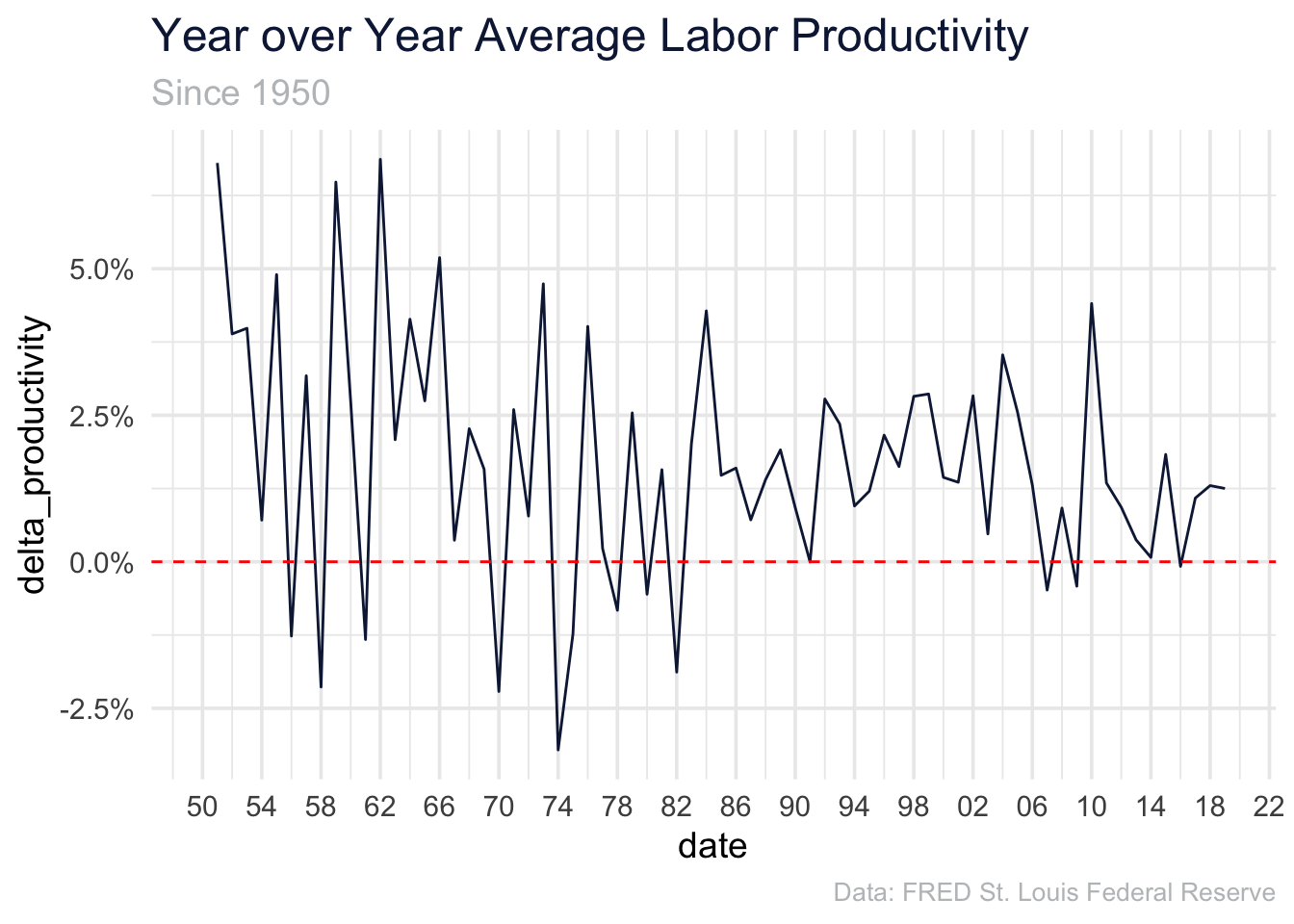

3.3 By Decade

If we want to aggregate these values and look at decade labor productivity growth, we can first filter our only the first and last years of the decade, and again calculate the percent change.

dat_decade_productivity <- dat_productivity %>% 
    group_by(decade = str_extract(year, "\\d{3}")) %>% 
    filter(year ==min(year) | year == max(year)) %>% 
    mutate(G = 1+ (productivity - lag(productivity, 1, default = 0))/lag(productivity, 1)) %>% 
    filter(!is.na(G)) %>% 
    mutate(g = G^(1/10)-1) %>% 
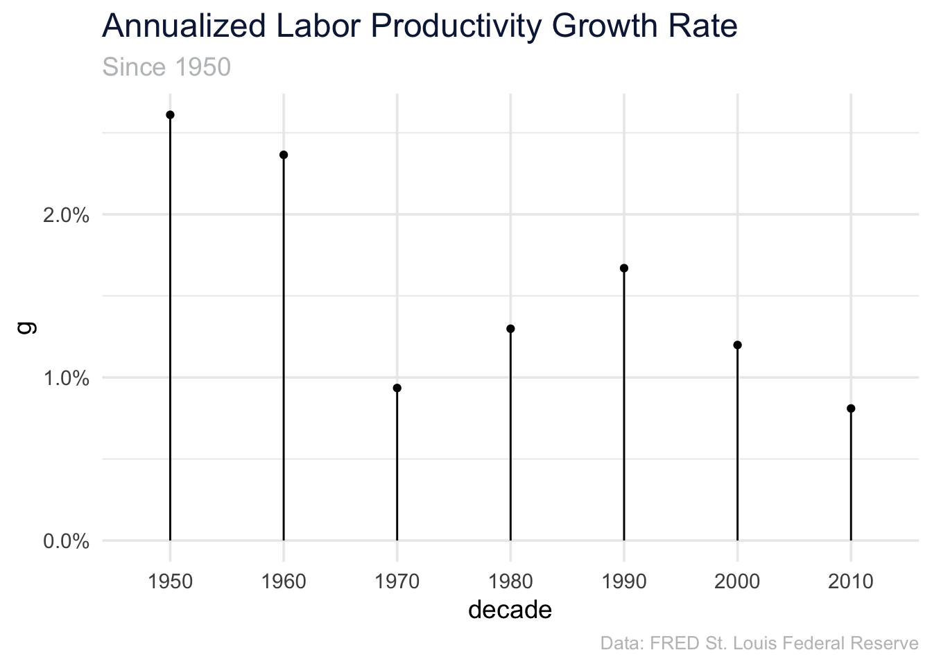
    ungroup()

3.3.1 Annualized Productivity

Finally, we often like to annualize percent change. In this case we can take our decade values and annualize them (to basically create an average year over year) labor productivity growth. This can be best represented by the below equation.

\[(1+g)^{10}=1+G\]

dat_decade_productivity %>% 
    mutate(decade = paste0(decade, "0")) %>% 
    ggplot(aes(x = decade, y = g)) +
    geom_point()+
    geom_segment(aes(yend = 0, xend = decade))+
    scale_y_continuous(labels = scales::percent)+
    labs(
        title = "Annualized Labor Productivity Growth Rate",
        subtitle = "Since 1950",
        caption = "Data: FRED St. Louis Federal Reserve"
    )

---

Intermediate Macroeconomics
me.dewitt.jr@gmail.com

Code licensed under the BSD 3-clause license
Text licensed under the CC-BY-ND-NC 4.0 license

See the Repository

Copyright © 2020 Michael DeWitt